Introduction
The DeltaMultipleBenefits package provides tools for estimating the net impacts of landscape changes in the Sacramento-San Joaquin River Delta on multiple metrics of interest to the Delta community. It provides models and data to support estimating the magnitude of potential multiple benefits and trade-offs resulting from changes to a baseline landscape. It can be used to estimate the effects of a proposed change to the landscape (e.g., habitat restoration plans) or anticipated changes to the landscape (e.g., agricultural crop conversion trends), individually or in combination with each other. It can be used to investigate the complex interactions among multiple drivers of landscape change and to facilitate discussions about alternative scenarios under consideration.
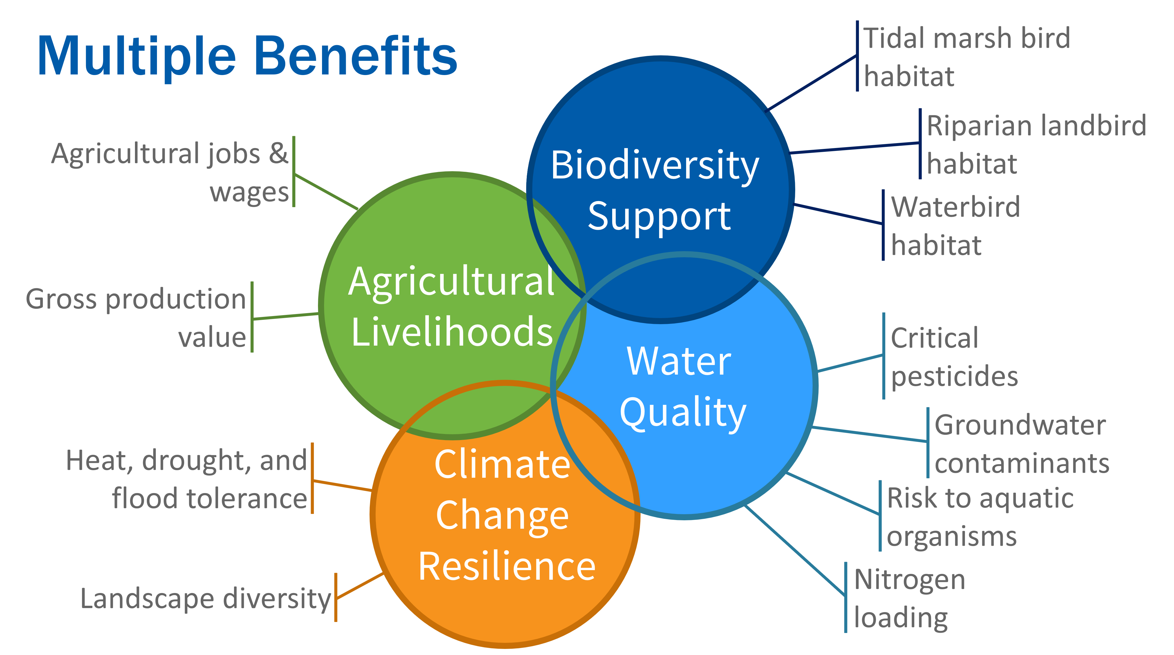
The metrics currently supported by this package are grouped into several categories of potential benefits: Agricultural Livelihoods, Water Quality, Climate Change Resilience, and Biodiversity Support. Each category is represented by multiple individual metrics that can be summarized over the entire landscape, regions within the landscape, or individual project areas. By comparing metrics estimated from proposed scenarios of landscape change to metrics estimated for a baseline landscape representing current conditions, the expected net change in each metric can be estimated.
Importantly, this package is not designed to find an “optimal” solution to maximize benefits and minimize trade-offs, but rather to evaluate and compare realistic proposed alternatives or anticipated future changes. This is because the list of supported metrics is incomplete compared to the many interests, values, and goals held by the Delta community, land managers, organizations, and agencies, so that any optimized solution would be incomplete and potentially misleading. Instead, this package requires users to supply spatial data representing their baseline (current) landscape and alternative scenarios under consideration. Example baseline and scenario landscapes used in the development of this package are publicly available for reuse or modification (see Supporting Information).
This vignette serves as a tutorial outlining the major steps of analyzing alternative landscapes and comparing them to each other, including:
- Preparing new landscape scenarios for analysis
- Summarizing the net change in the total area of each land cover class
- Estimating the net change in simple metrics
- Estimating the net change in metrics informed by spatial models
library(DeltaMultipleBenefits)
# library(sf)
# library(terra)
# library(dplyr)
# library(tidyr)
# library(ggplot2)
# library(tibble)
Step 1. Preparing a new landscape scenario for analysis
To prepare a new landscape scenario for analysis with the DeltaMultipleBenefits framework, its land cover classifications must first be aligned with those used in the framework, which are designed to work with the existing metrics and species distribution models. This land cover classification scheme includes both natural and agricultural land cover classes, and is organized hierarchically into major land cover classes and subclasses. Following Phase 2 of developing this package, we substantially updated the vegetation key to accommodate many more wetland vegetation suclasses.
data(key, package = 'DeltaMultipleBenefits')
head(key)
#> # A tibble: 6 × 7
#>   CODE_NUM CODE_NAME                  CLASS          SUBCLASS DETAIL LABEL COLOR
#>      <dbl> <chr>                      <chr>          <chr>    <chr>  <chr> <chr>
#> 1       10 AG_PERENNIAL               PERENNIAL CRO… NA       NA     Pere… #ECA…
#> 2       11 ORCHARD_DECIDUOUS          NA             DECIDUO… NA     Orch… #ECA…
#> 3       15 ORCHARD_CITRUS&SUBTROPICAL NA             CITRUS … NA     Orch… #ECA…
#> 4       19 VINEYARD                   NA             VINEYARD NA     Vine… #ECA…
#> 5       20 AG_ANNUAL                  ANNUAL CROPS   NA       NA     Annu… #F4C…
#> 6       21 GRAIN&HAY                  NA             GRAIN &… NA     Grai… #F4C…
We generally recommend assigning all land covers in your landscape scenario to the most specific subclass in the existing scheme as possible. Certain metrics and species distribution models will use individual subclasses, while others will lump them together into broader groupings.
1.1 Working with polygons
The most recent, comprehensive land cover and land use data set for
the Delta and Suisun Marsh that we are aware of is the
“Habitat_types_modern” provided in SFEI’s Landscape Scenario Planning
Tool v.3.0.0. To support alignment with this data set and its land cover
classification scheme, we developed the
classify_landcover.sf() function to support cross-walking
that layer to the land cover classes and subclasses required by the
models and metrics in this package. The result of this function is the
additon of fields representing the most detailed land cover class or
subclass that can be assigned according to the scheme provided in
key, as well as the corresponding predictors required to
fit the species distribution models supported by this package.
# EXAMPLE NOT RUN:
lspt <- sf::read_sf('path/to/Habitat_types_modern.shp')
lc_classified <- classify_landcover.sf(lspt)
Alternatively, and to work with other land cover data sources,
manually align land cover classes and subclasses with those provided in
key. As a toy example, and for further demonstrating the
additional steps in this vignette, we’ll work with the
olinda1 dataset provided with the sf package.
This data set includes place names instead of land cover
classifications, but we’ll treat them as though they represented land
covers and recode them to supported CODE_NAME values in the
key. Finally, we’ll join the key data to match
new CODE_NAME values to CODE_BASELINE values
we’ll need later on.
olinda1 <- sf::st_read(system.file("shape/olinda1.shp", package = "sf"),
quiet = TRUE) |>
sf::st_transform(26910)
head(olinda1)
#> Simple feature collection with 6 features and 6 fields
#> Geometry type: POLYGON
#> Dimension: XY
#> Bounding box: xmin: 16885570 ymin: -8723971 xmax: 16892730 ymax: -8717533
#> Projected CRS: NAD83 / UTM zone 10N
#> ID CD_GEOCODI TIPO CD_GEOCODB NM_BAIR V014
#> 1 28801 260960005000001 URBANO 260960005020 Ouro Preto 1119
#> 2 28802 260960005000002 URBANO 260960005020 Ouro Preto 1267
#> 3 28803 260960005000003 URBANO 260960005020 Ouro Preto 557
#> 4 28804 260960005000004 URBANO 260960005020 Ouro Preto 709
#> 5 28805 260960005000005 URBANO 260960005020 Ouro Preto 1045
#> 6 28806 260960005000006 URBANO 260960005020 Ouro Preto 727
#> geometry
#> 1 POLYGON ((16889505 -8717533...
#> 2 POLYGON ((16891561 -8719078...
#> 3 POLYGON ((16890240 -8721218...
#> 4 POLYGON ((16888737 -8722217...
#> 5 POLYGON ((16886823 -8722100...
#> 6 POLYGON ((16887682 -8720990...
new_shp <- olinda1 |>
# recode existing place name values with supported land cover names in key
dplyr::mutate(
CODE_NAME = dplyr::case_when(
NM_BAIR %in% c('Ouro Preto', 'Sítio Novo', 'Sapucaia', 'Salgadinho') ~
'ORCHARD_DECIDUOUS',
NM_BAIR %in% c('Tabajara', "Caixa D'Água", 'Águas Compridas',
'São Benedito') ~
'ORCHARD_CITRUS&SUBTROPICAL',
NM_BAIR %in% c('Fragoso', 'Alto da Bondade', 'Alto da Conquista',
'Passarinho') ~
'VINEYARD',
NM_BAIR %in% c('Bultrins', 'Jardim Atlântico', 'Rio Doce',
'Alto do Sol Nascente') ~
'GRAIN&HAY_WHEAT',
NM_BAIR %in% c('Alto da Nação', 'Monte', 'Casa Caiada') ~
'FIELD_CORN',
NM_BAIR %in% c('Guadalupe', 'Bonsucesso', 'Bairro Novo') ~
'RIPARIAN_FOREST_POFR',
NM_BAIR %in% c('Varadouro', 'Amparo', 'Amaro Branco') ~
'RIPARIAN_FOREST_QUER',
NM_BAIR %in% c('Vila Popular', 'Peixinhos', 'Carmo') ~
'WETLAND_TULE_CATTAIL_NONTIDAL',
NM_BAIR %in% c('Jardim Brasil', 'Aguazinha', 'Santa Teresa') ~
'WETLAND_PHRAGMITES_ARUNDO_TIDAL',
is.na(NM_BAIR) ~ 'PASTURE_ALFALFA',
TRUE ~ 'UNKNOWN')) |>
# transfer CODE_BASELINE values from key
dplyr::left_join(key |> dplyr::select(CODE_NUM, CODE_NAME, COLOR), by = 'CODE_NAME')
ggplot2::ggplot(new_shp) +
ggplot2::geom_sf(ggplot2::aes(fill = CODE_NAME))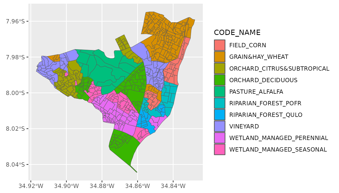 Next, convert the polygons to a raster format with the desired
projection, extent, and resolution. We’ll first create a raster template
from the polygon layer with a small number of columns and rows (and thus
coarse resolution) just for demonstration purposes. However, to ensure
alignment with other rasters in your analysis, it usually works best to
use an existing raster as a template. Next, transfer the land cover code
values to the template to create a new landscape raster that we’ll treat
as our “baseline” landscape. Finally, to help with plotting, we’ll
assign labels and default color codings to each value.
Next, convert the polygons to a raster format with the desired
projection, extent, and resolution. We’ll first create a raster template
from the polygon layer with a small number of columns and rows (and thus
coarse resolution) just for demonstration purposes. However, to ensure
alignment with other rasters in your analysis, it usually works best to
use an existing raster as a template. Next, transfer the land cover code
values to the template to create a new landscape raster that we’ll treat
as our “baseline” landscape. Finally, to help with plotting, we’ll
assign labels and default color codings to each value.
template = terra::rast(ncols = 1000, nrows = 1000,
                       extent = sf::st_bbox(new_shp))
terra::crs(template) = 'epsg:26910'
baseline = terra::rasterize(x = new_shp, y = template, field = 'CODE_NUM')
names(baseline) = 'baseline'

# assign factor levels:
levels(baseline) <-  key |>
  dplyr::select(CODE_NUM, CODE_NAME) |> as.data.frame()

# assign color coding
terra::coltab(baseline) <- key |>
  dplyr::select(CODE_NUM, COLOR) |> as.data.frame()
terra::plot(baseline)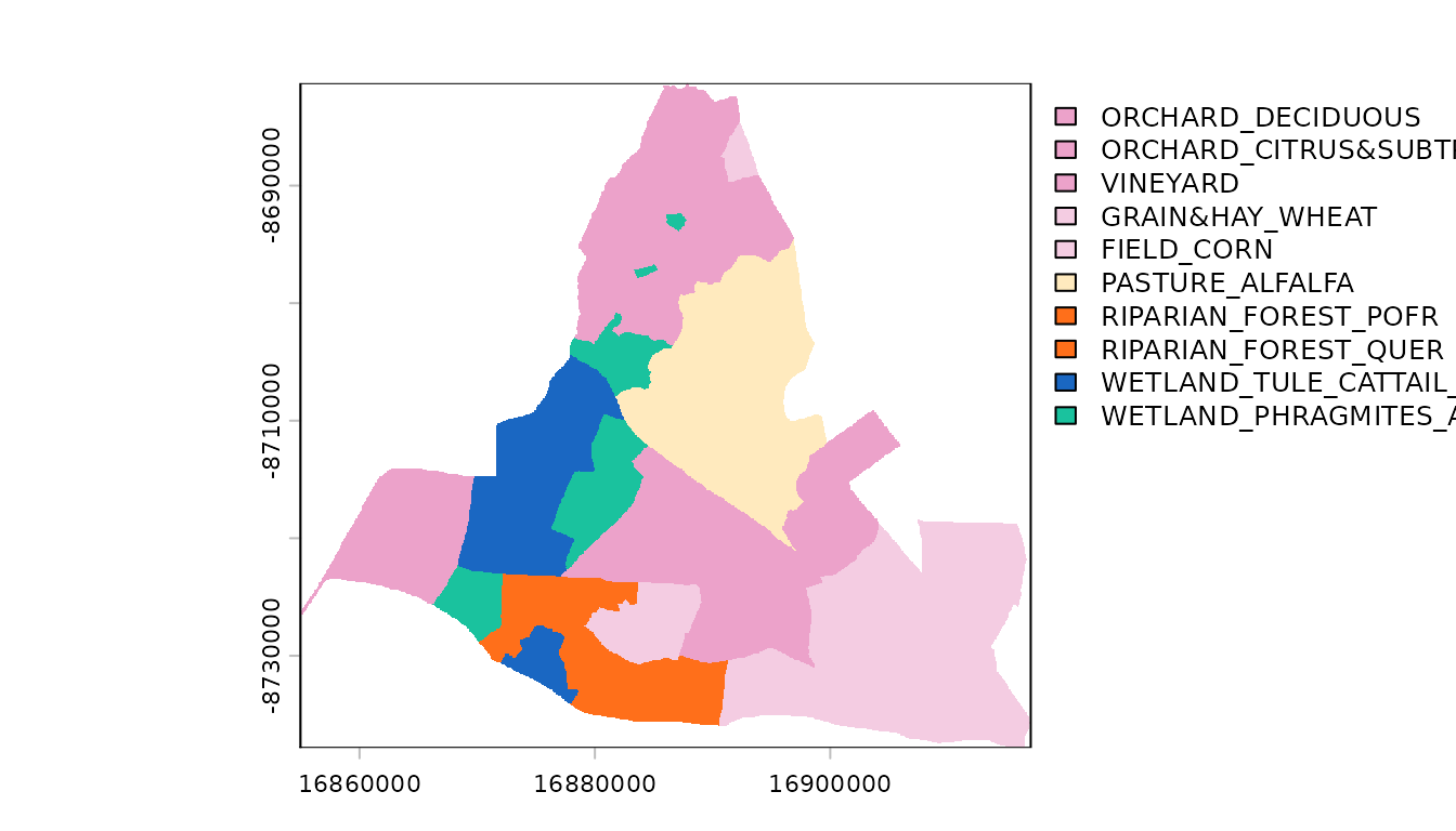
1.2 Working with existing rasters
If the landscape to be analyzed is in a raster format already, the
existing land cover values encoded should be similarly translated to the
supported values in the existing land cover classification scheme. As an
example, we’ll use baseline raster we created above, and
create a new version from it to serve as our new scenario
of landscape change.
# basic example habitat restoration scenario: all wheat (22) and corn (26)
# pixels are converted to Fremont cottonwood riparian forest (71)
scenario <- terra::classify(
  baseline,
  rcl = data.frame(from = c(22, 26),
                   to = c(71, 71)) |> as.matrix())
levels(scenario) <- key |>
  dplyr::select(CODE_NUM, CODE_NAME) |> as.data.frame()
terra::coltab(scenario) <- key |>
  dplyr::select(CODE_NUM, COLOR) |> as.data.frame()

# stack landscapes to compare
landscapes = c(baseline, scenario)
names(landscapes) = c('baseline', 'scenario')
terra::plot(landscapes) 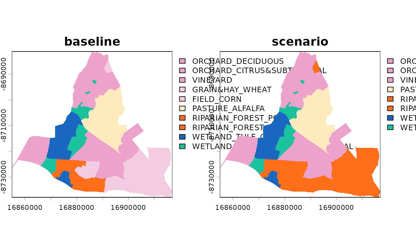
# Note the light pink wheat and corn cells have changed to orange-red riparian
# cells
rm(baseline, scenario, olinda1, key)
Step 2. Summarizing the net change in the total area of each land cover class
Built-in functions make it simple to estimate the change in the total area of each land cover class between the baseline and one or more scenario landscape rasters. First, sum the total area of each land cover class in each landscape raster, then summarize the change between them.
sum_landcover: This function takes a SpatRaster with
one or more layers and, for each layer, counts the number of pixels of
each unique land cover class and multiplies by the provided
pixel_area value to estimate the total area of each land
cover class. It returns a tibble with the scenario name (taken from the
names of each raster layer), the CODE_NAME of each land
cover class, and the total area. Here we’ll first use
terra::cellSize to estimate the area of each pixel in ha.
The option rollup = TRUE adds extra rows to the output with
the sum total area for all riparian and wetland subclasses. This
function also supports options to mask out portions of the raster and/or
to summarize the total area by zones or regions within the
landscape.
units = 'ha'

area = terra::cellSize(landscapes, unit = units)[50,50] |> tibble::deframe()

landcover_totals = sum_landcover(
  landscapes = landscapes,
  pixel_area = area,
  rollup = TRUE,
  zones = NULL) |>
  dplyr::arrange(scenario, CODE_NAME) |>
  dplyr::mutate(units = units)
head(landcover_totals)
sum_change: This function calculates the net change
in the area of each land cover class between the baseline landscape and
one or more scenario landscapes. Note that this function expects the
output from sum_landcover, which includes the field
scenario representing the names of each landscape. At least
one scenario must be named “baseline”, and all other scenarios will be
assumed to represent an alternative scenario landscape for comparison to
the baseline. Thus the net change for multiple scenarios can be
estimated simultaneously. The result is a tibble with the scenario name,
the CODE_NAME of each land cover class, fields representing
the total area of the land cover class for the scenario in question and
the corresponding area for the baseline, and then the
net_change between them, where a positive value indicates
an increase from the baseline.
landcover_change = sum_change(landcover_totals)
head(landcover_change)
# Note net increase in riparian (and specifically POFR) and decrease in wheat and corn, as expected.
Step 3. Estimating the net change in simple metrics
The DeltaMultipleBenefits package supports evaluation of
several relatively “simple” metrics representing the benefits
categories: agricultural livelihoods, water quality,
and climate change resilience. For example, agricultural
livelihood metrics include the number of agricultural jobs, their
average annual wage, and gross production value. These are all “simple”
metrics in the sense that a single mean value for each metric is used to
represent each land cover class, regardless of where in the Delta the
land cover is located. Therefore, estimating the net change in these
metrics between a baseline and scenario landscape is relatively simple
compared to estimating the net change in metrics derived from a spatial
model (see below). The steps for estimating the net change in these
simple metrics are similar to estimating the net change in land cover
area above. However, the uncertainty in the value of each metric for
each land cover class (where available) is also accounted for in
estimating the uncertainty in the net change.
The values assigned to each land cover class for each metric are included in this package, and are also published and available to download separately (see Supporting Information). However, these metrics can be edited to provide updated values or custom additional metrics as needed.
sum_metrics: First estimate the total landscape
score for each metric and landscape raster, by combining total area of
each land cover class estimated above with the per-unit-area metrics for
each land cover class. For most metrics, this involves multiplying the
per-unit-area metrics by the total area of each land cover class and
summing over the entire landscape. For Annual Wages (as part of the
Agricultural Livelihoods category of benefits), it instead calculates
the new weighted average wage across all agricultural hectares (i.e.,
those supporting agricultural jobs with an associated wage value). For
metrics in the Climate Change Resilience category, it instead calculates
the new overall average resilience score on a scale of 1 (low
resilience) to 10 (high resilience). The function returns a tibble with
the scenario name, fields from metrics defining metric
categories and units, a SCORE_TOTAL and a
SCORE_TOTAL_SE, representing the combined uncertainty. The
units field is also updated to reflect that the scores are
no longer per-hectare, but instead summed over all hectares in the
landscape.
The total area of each land cover class as calculated above includes
both the area of individual riparian and managed wetland subclasses as
well as the roll-up total area (because we used
rollup = TRUE), so we must take care not to double-count
them in the total landscape scores calcualted here. Thus far, these
simple metrics are not specific to individual riparian and
wetland subclasses and instead apply to riparian and wetland land covers
generally. Therefore, here we filter out the subclasses to exclude them
from this calculation.
Note: We will get a warning message here, because our toy example landscape does not include all land cover classes present in our metrics data.
scores = sum_metrics(
  metricdat = metrics,
  areadat = landcover_totals |> dplyr::filter(!(grepl('RIPARIAN_|WETLAND_', CODE_NAME))))
head(scores)
sum_change: Then, we can again use
sum_change to estimate the difference in each metric
between the baseline and scenario landscapes. However, this time because
there is uncertainty in the total landscape scores, the uncertainty in
the difference will also be estimated. Here we use a coverage factor
k = 2 to approximate a 95% confidence interval for the
net_change.
scores_change = sum_change(scores, k = 2)
head(scores_change)
Visualize the resulting estimates of net change: (Note no error bar for N loading due to lack of uncertainty estimates)
scores_change |>
  dplyr::mutate(
    # invert water quality scores so a reduction in pesticide use is shown as a
    # net benefit
    net_change = dplyr::if_else(
      METRIC_CATEGORY == 'Water Quality', -1 * net_change, net_change),
    # rescale scores and confidence intervals with very large numbers to facilitate
    # comparisons
    dplyr::across(
      c(net_change, lcl, ucl),
      ~dplyr::case_when(
             METRIC == 'Gross Production Value' ~ .x/1000,
             METRIC == 'N loading' ~ .x/1000,
             TRUE ~ .x))
    ) |>
  ggplot2::ggplot(ggplot2::aes(net_change, METRIC)) +
  ggplot2::facet_wrap(~METRIC_CATEGORY, ncol = 1, scales = 'free') +
  ggplot2::geom_col(fill = 'gray80') +
  ggplot2::geom_errorbar(ggplot2::aes(xmin = lcl, xmax = ucl), width = 0.25) +
  # add blank geoms to ensure zeroes line up across facets
  ggplot2::geom_blank(ggplot2::aes(x = -ucl)) +
  ggplot2::geom_blank(ggplot2::aes(x = -lcl)) +
  ggplot2::theme_minimal()
Step 4. Estimating the net change in metrics informed by spatial models
In addition to the “simple” metrics described above, the
DeltaMultipleBenefits package supports evaluation of more
complex spatial models that consider not only the total extent of each
land cover class in the landscape but also their spatial configuration.
For example, whether or not an area is suitable habitat for wildlife
species often depends on both the local land cover class as well as the
surrounding land cover classes and proximity to specific features on the
landscape (such as distance to a water channel). Evaluating the net
change in these metrics between scenario and baseline landscapes is
necessarily more complicated than evaluating the “simple” metrics above,
but also allows for more nuance and spatial variation within the
landscape.
The package currently supports application of several species distribution models for birds to represent the Biodiversity Support benefits category, with metrics that represent the estimated extent of suitable habitat for each species or group of species. These include 3 sets of models: * “riparian”: 9 riparian landbird species during the breeding season * “waterbird_fall”: 6 groups of waterbird species during the fall season * “waterbird_win”: 6 groups of waterbird species during the winter season * “tima”: 7 tidal marsh bird species, including 3 secretive marsh bird species and 4 tidal wetland songbird species
See Supporting Information for links to manuscripts and reports describing the development of these models and links to download the R data files containing these models (they are not provided within the R package due to their size).
Spatial models for other species, other benefits categories and metrics, and/or to represent the “simple” metrics in a more nuanced, spatially-dependent way could be incorporated in future versions of this package. Please contact us to suggest future extensions of this package and to collaborate on further development.
All of these species distribution models include predictors representing local land cover statistics (e.g., proportion cover within 100m) and predictors representing the surrounding landscape (e.g., proportion cover within 2km). However, the land cover classes and subclasses most relevant to each group of species vary, while other land cover classes may be lumped together into a single predictor. Therefore, to apply these species distribution models to new baseline and scenario landscapes, the land cover classes must be first cross-walked to the relevant predictors for each set of models. Then, focal statistics must be run using the moving window sizes relevant to each set of models. Finally, additional predictors specific to individual sets of models may also need updating. Here, we walk through the key steps necessary for each set of models.
4.1 Tidal marsh bird models (“tima”)
The models developed in Phase 2 include 7 tidal wetland focal species: 3 secretive marsh bird species (California Black Rail, American Bittern, and Least Bittern), as well as 4 tidal marsh songbird species (Common Yellowthroat, Marsh Wren, Song Sparrow, and Yellow-breasted Chat).
4.1.1 Prepare landscape predictors
To apply the “tima” models to new baseline and scenario landscapes, first use built-in functions to prepare the landscape rasters.
python_focal_prep: The first step is to prepare the
landscape rasters for calculating focal stats by reclassifying them to
match the predictor groupings required by the “tima” models and
separating them into layers representing each distinct predictor, with a
default value of 1 everywhere the land cover class is
present, and a 0 otherwise. The result can be optionally
directly written to a directory located at:
dir/SDM/landscape_name where landscape_name is
taken from the name(s) of the input SpatRaster. If the directory does
not already exist, it will be created automatically.
estimate_tima_patchsize: From the results, we’ll also estimate the size of contiguous patches of tidal wetland vegetation.
Note: We will get warning messages here, because our toy example landscape does not include all land cover classes required to fit the “tima” models.
predictors_tima = python_focal_prep(landscapes, SDM = 'tima', dir = 'example',
                                    fill = FALSE) |> suppressWarnings()

psize = estimate_tima_patchsize(predictors_tima, dir = 'example')

terra::plot(c(predictors_tima$baseline$TWET, psize[[1]]))
rasterize_stream_channels: To facilitate estimating
the density (proportion cover) of channel lines, we also need to compile
water channel data, based on the California Aquatic Resources Inventory
(CARI) Streams (lines) data set. These data are freely available for
download from SFEI
and CDFW.
Download these data first, and then either provide the path to the
shapefile or file geodatabase, or provide the sf object
directly. By default, this layer will be considered the “baseline”
representation of stream channels. However, it can also be applied to
alternative scenarios if stream channel locations will not change by
giving a different landscape_name, or the result of this
function can be manipulated to represent changes to channel locations
under alternative scenarios.
chan = rasterize_stream_channels(
  x = 'path/to/cari_streams', template = predictors_tima$baseline,
  min_length = 1, dir = 'example',
  landscape_name = 'baseline')
python_focal_stats: The next step is to generate focal statistics for each of the separate rasters generated in the previous steps that represent land cover predictors, tidal wetland patch size, and stream channel locations. Focal statistics perform a given operation on all cells within a given distance of the focal cell, and repeated for every cell in the raster.
For the “tima” models, this function will calculate the mean value
for the presence of every raster layer in
pathin/SDM/landscape_name within moving windows on each of
two spatial scales (50m and 2km). The function must be run a second time
to with regex = 'PSIZE.tif' and
overwrite = TRUE to replace the mean value of the tidal
marsh patch size within each spatial scale with the maximum value. All
results are written directly to dir/SDM/landscape_name and
not returned to working memory.
These calculations can be very slow, depending on the size and
resolution of the rasters. To enhance processing speed, this function
currently requires Python to be installed on your system and
specifically arcpy with the Spatial Analyst extension. The
first time this function is run in each session, internal helper
functions will check that arcpy is installed and try to
load it, but to ensure the correct version of Python can be found, you
may need to specify the correct filepath.
python_focal_stats(SDM = 'tima',
                   landscape_names = c('baseline', 'scenario'),
                   pathin = 'example',
                   dir = 'SDM_predictors')

python_focal_stats(SDM = 'tima',
                   landscape_names = c('baseline', 'scenario'),
                   pathin = 'example',
                   dir = 'SDM_predictors',
                   regex = 'PSIZE.tif',
                   overwrite = TRUE)
update_covertype: Finally, covertype is a
categorical predictor reflecting the land cover class in each pixel. The
original bird survey data used to develop these models only included a
subset of available land cover classes, and these classes had an
influence on the probability of species presence: wetland, riparian,
water, and a combined group of annual agricultural crops, idle fields,
grassland, and ruderal (non-woody) vegetation. This function extracts
these landcovers from the input SpatRasters and creates a
“LANDCOVER.tif” layer ready to use in the distribution models. It can be
written to the same output directory as the results from running
python_focal_stats() above.
covertype_tima = update_covertype(landscapes, SDM = "tima", dir = 'SDM_predictors')
terra::plot(covertype_tima)
4.1.2 Generate model predictions
fit_SDM: Use the predictors created in the previous
step for each landscape to fit the distribution models for each of the 7
“tima” species. The modlist should refer to an R object
containing a list of the tidal marsh distribution models. See Supporting Information
to download these models. The levels of the categorical predictor
LANDCOVER must be specified in the call to
fit_SDM, and in the correct order.
Open water was considered to be an unsuitable land cover class a
priori, and so we can specify unsuitable = 90 (the
land cover class value for open water); this will create a mask from the
provided landscape with 0 values wherever the land cover
class equals the values provided in unsuitable and NA
elsewhere, used to cover the predicted values from the model.
Alternatively, the predictors can all be masked by an open water layer
before running fit_SDM().
fit_SDM(pathin = 'SDM_predictors',
        SDM = 'tima',
        landscape_name = 'baseline',
        modlist = BRT_tidal_wetlands,
        factors = list(list('LANDCOVER' = c('WETLAND', 'RIPARIAN', 'WATER', 'AGGRPAS'))),
        type = 'response',
        unsuitable = 90,
        dir = 'SDM_results')

fit_SDM(pathin = 'SDM_predictors',
        SDM = 'tima',
        landscape_name = 'scenario',
        modlist = BRT_tidal_wetlands,
        factors = list(list('LANDCOVER' = c('WETLAND', 'RIPARIAN', 'WATER', 'AGGRPAS'))),
        type = 'response',
        unsuitable = 90,
        dir = 'SDM_results')
Note: The models will not run if all required predictors are not provided. The toy example landscape data provided here does not include all required predictors.
transform_SDM: The model-predicted results can be
converted into binary presence-absence predictions using threshold
statistics derived from the dismo::threshold function.
Here, we use the statistic equal_sens_spec, which is the
value at which specificity (the probability of correctly predicting
species absence) is equal to sensitivity (the probability of correctly
predicting species presence), but other statistics can be selected (see
?dismo::threshold).
transform_SDM(pathin = 'SDM_results',
              SDM = 'tima', landscape_name = 'baseline',
              modlist = BRT_tidal_wetlands,
              stat = 'equal_sens_spec',
              dir = 'SDM_results_threshold')

transform_SDM(pathin = 'SDM_results',
              SDM = 'tima', landscape_name = 'scenario',
              modlist = BRT_tidal_wetlands,
              stat = 'equal_sens_spec',
              dir = 'SDM_results_threshold')
4.2 Riparian landbird models (“riparian”)
The models developed in Phase 1 include 9 riparian landbird species, including 3 of the same species also addressed in Phase 2 for tidal wetlands: Common Yellowthroat, Marsh Wren, Song Sparrow, and Yellow-breasted Chat, as well as: Nuttall’s Woodpecker, Ash-throated Flycatcher, Black-headed Grosbeak, Lazuli Bunting, Yellow Warbler, and Spotted Towhee. These models were built for the entire Central Valley and focused on riparian vegetation and did not include as much wetland vegetation detail as the Phase 2 models. Thus, we now recommend using the Phase 2 models for those species, and Phase 1 models for the rest.
4.2.1 Prepare landscape predictors
To apply the “riparian” models to new baseline and scenario landscapes, the process is very similar to that for “tima” demonstrated above, with a few exceptions.
classify_landcover & python_focal_prep: The
first step is again to prepare for focal statistics, including by
creating the predictor groupings required by the “riparian” models. In
this case, it is best to work directly with the original LSPT
Habitat_types_modern layer, if possible. The
classify_landcover.sf() function applied to the LSPT data
will return the corresponding predictors for the “riparian” models with
the greatest accuracy and specificity. Then the call to
python_focal_prep() can include
classified = TRUE to bypass the internal call to
classify_landcover.SpatRaster(). To demonstrate:
lspt <- sf::read_sf('path/to/Habitat_types_modern.shp')
lc_classified <- classify_landcover.sf(lspt)
baseline_rip = terra::rasterize(x = lc_classified, y = template,
                                field = 'PREDICTOR_RIPARIAN')
scenario_rip <- terra::classify(
  baseline_rip,
  rcl = data.frame(from = c(22, 26),
                   to = c(71, 71)) |> as.matrix())
landscapes_rip = c(baseline_rip, scenario_rip)
names(landscapes_rip) = c('baseline', 'scenario')

predictors_rip = python_focal_prep(landscapes, SDM = 'riparian', dir = 'example',
                                   fill = FALSE, classified = TRUE) |> suppressWarnings()
Otherwise, python_focal_prep() can still be called
directly (with classified = FALSE), but the internal call
to classify_landcover.SpatRaster()may produce some minor
differences from the original land cover classification scheme used in
the development of these models. Note that these layers can be written
to the same dir as the ‘tima’ models above, but they will
be kept in a separate subdirectory for the ‘riparian’ SDMs.
predictors_rip = python_focal_prep(landscapes, SDM = 'riparian', dir = 'example',
                                   fill = FALSE) |> suppressWarnings()

terra::plot(predictors_rip$baseline)
python_focal_stats: As above, the next step is to generate focal statistics for each of the separate land cover rasters.
python_focal_stats(SDM = 'riparian',
                   landscape_names = c('baseline', 'scenario'),
                   pathin = 'example',
                   dir = 'SDM_predictors')
4.2.2 Prepare additional predictors
The “riparian” models also include several predictors not based on
land cover data: - area.ha, accounting for variation in
survey effort, which should be held constant for new predictions; -
region, indicating whether the survey was conducted in the
Sacramento Valley (region = 0) or in the Delta or San Joaquin (region =
1) - bio_1, representing annual mean temperature, 1970-2000
- bio_12, representing total annual precipitation,
1970-2000 - streamdist, representing the square-root of the
distance (in m) to the nearest stream or river, based on the National
Hydrography Dataset
To represent area.ha in new predictions, we recommend
using a constant value of 3.14159, referring to the total area (in
hectares) within 50m of a bird survey location, after 4 surveys. For
region, we recommend using a constant value of 1 for
predictions in the Delta. These constant values can be called directly
in the fit_SDM() function below.
For bio_1, bio_12, and
streamdist, see Supporting Information
to download the original layers used in developing these models. They
can be added directly to the same directory containing the land cover
predictors for use in fitting the SDMs, though they may need to be
cropped and aligned with the other rasters first.
4.2.3 Generate model predictions
fit_SDM: Once all required predictors are
represented, the next step is to fit the distribution models for each of
the 9 “riparian” species. Alternatively, only include the 6 species not
already represented by the “tima” models. As above, see Supporting Information
to download these models. Note that, in the original analysis open water
was considered to be an unsuitable land cover class for riparian
landbirds a priori, and so we can specify
unsuitable = 90 (the land cover class value for open
water); this will create a mask from the provided landscape
with 0 values wherever the land cover class equals the values provided
in unsuitable and NA elsewhere, used to cover the predicted
values from the model.
transform_SDM: Finally, as above, the model-predicted results can be converted into binary presence-absence predictions using threshold statistics.
# baseline landscape:
fit_SDM(pathin = 'SDM_predictors',
        SDM = 'riparian',
        landscape_name = 'baseline',
        modlist = BRT_riparian_wetlands[[c('NUWO', 'ATFL', 'BHGR', 'LAZB', 'SPTO', 'YEWA')]],
        constants = data.frame(region = 1,
                               area.ha = 3.141593),
        unsuitable = 90, #open water
        dir = 'SDM_results')

transform_SDM(pathin = 'SDM_results',
              SDM = 'riparian', landscape_name = 'baseline',
              modlist = BRT_riparian_wetlands[[c('NUWO', 'ATFL', 'BHGR', 'LAZB', 'SPTO', 'YEWA')]],
              stat = 'equal_sens_spec',
              dir = 'SDM_results_threshold')

# scenario landscape:
fit_SDM(pathin = 'SDM_predictors',
        SDM = 'riparian',
        landscape_name = 'scenario',
        modlist = BRT_riparian_wetlands[[c('NUWO', 'ATFL', 'BHGR', 'LAZB', 'SPTO', 'YEWA')]],
        constants = data.frame(region = 1,
                               area.ha = 3.141593),
        unsuitable = 90, #open water
        dir = 'SDM_results')

transform_SDM(pathin = 'SDM_results',
              SDM = 'tima', landscape_name = 'scenario',
              modlist = BRT_riparian_wetlands[[c('NUWO', 'ATFL', 'BHGR', 'LAZB', 'SPTO', 'YEWA')]],
              stat = 'equal_sens_spec',
              dir = 'SDM_results_threshold')
4.3 Waterbird models (“waterbird_fall” and “waterbird_win”)
The models developed in Phase 1 also include 5 groups of waterbird species during the fall season (July - mid-Nov) and 6 groups during the winter (mid-Nov - Mar): geese, dabbling ducks, diving ducks (winter only), cranes, shorebirds, and herons/egrets. The two seasons represent the changes in species abundance during the non-breeding season as well as changes in land cover, especially specific crop classes in areas where there is a distinct winter crop. Therefore, fitting these models requires season-specific baseline and scenario landscapes.
4.3.1 Prepare landscape predictors
update_pwater: To apply the “waterbird_fall” and
“waterbird_win” models to new baseline and scenario landscapes, first
handle changes in the probability of surface water. The waterbird
distribution models included pwater, a predictor indicating
the probability of surface water during each season. It was included
both as a direct predictor (i.e. at each pixel or survey location) and
as the proportion of each land cover class surrounding each pixel or
survey location that was flooded, This function is used to create
estimates of pwater for portions of the alternative scenario landscapes
that have changed land cover class, and therefore may have changed in
the probability of surface water. The new predicted value for
pwater assigned to these areas is based on rasters
representing baseline land cover classes and corresponding baseline
historical flooding averages during the relevant season to calculate the
average historical flooding probability by land cover class. See Supporting Information
to download the original historical flooding data used in developing
these models; substantial changes in land cover or flooding patterns may
require updating to more current flooding data. Here, for illustration
purposes, we randomly generate an example baseline pwater
for each season and then use the function to create an updated
pwater layer for our example scenario.
pwater_base_fall = terra::rast(
  landscapes$baseline,
  vals = runif(terra::ncell(landscapes$baseline), min = 0, max = 1))
pwater_scenario_fall = update_pwater(
  waterdat = pwater_base_fall, SDM = 'waterbird_fall',
  landscape_name = 'scenario',
  mask = landscapes$baseline,
  dir_focal = 'example', dir_final = 'SDM_predictors',
  baseline_landscape = landscapes$baseline,
  scenario_landscape = landscapes$scenario,
  floor = FALSE,
  overwrite = TRUE)
pwater_fall = c(pwater_base_fall, pwater_scenario_fall)
names(pwater_fall) = c('baseline', 'scenario')

# repeat for winter
pwater_base_win = terra::rast(
  landscapes$baseline,
  vals = runif(terra::ncell(landscapes$baseline), min = 0, max = 1))
pwater_scenario_win = update_pwater(
  waterdat = pwater_base_win, SDM = 'waterbird_win',
  landscape_name = 'scenario',
  mask = landscapes$baseline,
  dir_focal = 'example', dir_final = 'SDM_predictors',
  baseline_landscape = landscapes$baseline,
  scenario_landscape = landscapes$scenario,
  floor = FALSE,
  overwrite = TRUE)
pwater_win = c(pwater_base_win, pwater_scenario_win)
names(pwater_win) = c('baseline', 'scenario')
python_focal_prep: Now use built-in functions to
prepare the remaining landscape rasters, as above, this time
incorporating the updated pwater estimates. By providing a
pixel_value, cells where each land cover class is present
will be filled with a value corresponding to the area of each pixel (for
use in summing the total area of each land cover class with focal
statistics). In addition, by providing the pwater data as a
subset, the pwater layer will be masked by
each land cover class, resulting in a second set of layers filled with
values corresponding to their probability of being flooded. Because two
layers are created to represent each land cover class, two custom
suffix values must be provided to distinguish them when the
files are written to dir/SDM/landscape_name.
Note: If we had changes in crop class between the fall and winter
seasons, we would need to generate a winter version of the
landscapes data to analyze.
predictors_watfall = python_focal_prep(
  landscapes, SDM = 'waterbird_fall', dir = 'example', fill = FALSE,
  subset = pwater_fall, pixel_value = 0.09, suffix = c('_area', '_pfld')) |>
  suppressWarnings()

predictors_watwin = python_focal_prep(
  landscapes, SDM = 'waterbird_win', dir = 'example', fill = FALSE,
  subset = pwater_win, pixel_value = 0.09, suffix = c('_area', '_pfld')) |>
  suppressWarnings()
python_focal_stats: As above, the next step is to generate focal statistics for each of the separate land cover rasters.
python_focal_stats(SDM = 'waterbird_fall',
                   landscape_names = c('baseline', 'scenario'),
                   pathin = 'example',
                   dir = 'SDM_predictors')

python_focal_stats(SDM = 'waterbird_win',
                   landscape_names = c('scenario', 'scenario'),
                   pathin = 'example',
                   dir = 'SDM_predictors')
4.3.2 Prepare additional predictors
update_roosts & python_dist: In addition to changes in the probability of open water on the landscape, land cover changes may also affect the suitability of traditional night-time crane roosts. Because the distance to roost was an important predictor on the distribution models for cranes, accounting for the loss of traditional roost locations would affect these distances. The original data source for traditional roost locations is included in this package, but could be combined with updated information as it becomes available.
The update_roosts function allows defining which land
cover class codes are incompatible with crane roosts, and the threshold
proportion of the traditional crane roost polygon at which the entire
roost would be considered unsuitable. In our original analyses, we
considered crane roosts to be incompatible with perennial crops, urban
land cover, riparian vegetation, woodland, or scrub, and we assumed once
20% of the roost was covered by unsuitable land covers, the roost
location would be abandoned. The result of update_roosts is
an intermediate file at representing the new assumed locations of
traditional roosts, which is then used as an input to
python_dist for use in updating the estimated distance to
roost predictor for each pixel in the landscape.
Note: The land cover types we have designated as “unsuitable” for use as a crane roost are not expected to vary seasonally, and so we do not need to create separate versions corresponding to fall and winter waterbird SDMs.
data(roosts_original)

update_roosts(
  landscape = landscapes$scenario,
  roosts = terra::vect(roosts_original),
  filename = 'example/roosts/roosts.tif')

droost = python_dist(
  x = roosts,
  scale = 'km',
  dir = 'SDM_predictors',
  SDM = c('waterbird_fall', 'waterbird_win'), # can write to more than one location
  landscape_name = 'scenario',
  filename = 'droost_km.tif')
update_covertype: Like the “tima” models, these models include a categorical cover type predictor
covertype_watfall = update_covertype(landscapes, SDM = "waterbird_fall",
                                     dir = 'SDM_predictors')
terra::plot(covertype_watfall)

covertype_watwin = update_covertype(landscapes, SDM = "waterbird_win",
                                    dir = 'SDM_predictors')
terra::plot(covertype_watwin)
4.3.3 Generate model predictions
fit_SDM: Once all required predictors are
represented, the next step is to fit the distribution models for each of
the 5 fall waterbird groups and6 winter waterbird groups. As above, see
Supporting
Information to download these models. Similar to the “tima” models,
the levels of the categorical predictor covertype must be
specified in the call to fit_SDM, and in the correct order;
note that the factor levels change between fall and winter seasons. In
the original analysis perennial crops, urban, and barren land covers
were considered to be unsuitable land cover classes a priori,
and so we can specify unsuitable = c(10:19, 60, 130) (the
corresponding land cover class values).
Also similar to the riparian models, the waterbird models included
offset, a predictor accounting for variation in survey
effort, with different values applied to the predictions for waterbird
groups in fall vs. winter, as well as a separate value for cranes and
geese during the fall (which had a more restricted fall season). Thus,
due to the distinct values for offset, call
fit_SDM three times.
transform_SDM: Finally, as above, the model-predicted results can be converted into binary presence-absence predictions using threshold statistics.
# fall: cranes, geese
purrr::map(names(landscapes),
           ~fit_SDM(
             pathin = 'SDM_predictors',
             SDM = 'waterbird_fall',
             landscape_name = .x,
             modlist = waterbird_mods_fall[c('crane', 'geese')],
             constants = data.frame(offset = 3.709),
             factors = list(list('covertype' = c('Alfalfa',
                                                 'Irrigated pasture',
                                                 'Rice',
                                                 'Wetland'))),
             unsuitable = c(10:19, 60, 130),
             landscape = landscapes[[.x]],
             dir = 'SDM_results'))

# fall: dblr, shore, cicon:
purrr::map(names(landscapes),
           ~fit_SDM(
             pathin = 'SDM_predictors',
             SDM = 'waterbird_fall',
             landscape_name = .x,
             modlist = waterbird_mods_fall[c('dblr', 'cicon', 'shore')],
             constants = data.frame(offset = 4.435),
             factors = list(list('covertype' = c('Alfalfa',
                                                 'Irrigated pasture',
                                                 'Rice',
                                                 'Wetland'))),
             unsuitable = c(10:19, 60, 130),
             landscape = landscapes[[.x]],
             dir = 'SDM_results'))

# winter: all
purrr::map(names(landscapes),
           ~fit_SDM(
             pathin = 'SDM_predictors',
             SDM = 'waterbird_win',
             landscape_name = .x,
             modlist = waterbird_mods_win,
             constants = data.frame(offset = 3.617),
             factors = list(list('covertype' = c('Alfalfa',
                                                 'Corn',
                                                 'Irrigated pasture',
                                                 'Rice',
                                                 'Wetland',
                                                 'Winter wheat'))),
             unsuitable = c(10:19, 60, 130), #perennial crops, urban, barren
             landscape = scenarios[[.x]],
             dir = 'SDM_results',
             overwrite = TRUE))
transform_SDM: Again, as with riparian landbirds, convert the continuous probabilities of waterbird group presence predicted in the previous step to binary predictions of presence or absence.
purrr::map(names(landscapes),
           ~transform_SDM(
             pathin = 'SDM_results',
             SDM = 'waterbird_fall',
             landscape_name = .x,
             modlist = BRT_riparian[1],
             stat = 'equal_sens_spec',
             dir = 'SDM_results_threshold'))

purrr::map(names(landscapes),
           ~transform_SDM(
             pathin = 'SDM_results',
             SDM = 'waterbird_win',
             landscape_name = .x,
             modlist = BRT_riparian[1],
             stat = 'equal_sens_spec',
             dir = 'SDM_results_threshold'))
4.4 Estimate the net change in bird habitat
At this stage, the steps for estimating the net change in the total amount of habitat provided by each scenario for riparian landbirds and waterbird groups is similar to estimating the net change in the area of each land cover class and in each of the “simple metrics” above.
sum_habitat: Estimate the total area of each
landscape each species is predicted to occupy. This function is similar
to sum_landcover, but with a few key differences. By
default, all prediction rasters in the pathin argument and
any subdirectories will be included, so it can handle the results from
multiple scenarios and multiple sets of distribution models
simultaneously. However, SDM or both SDM and
landscape_name can optionally be specified to limit the
predictions evaluated. In addition, by including the option
rollup = TRUE, the total area occupied by at least one
species in the set will also be calculated.
By default, the result is the total count of pixels with a predicted
species presence, but the count can be optionally multiplied by the area
of each pixel by providing a pixel_area value in the
desired units. Here we also added a mutate argument to the
results to clearly specify the units used. Either way, the results are
structured to align with the results of sum_metrics() used
above for summarizing the total landscapes scores for the simple
metrics, so that the habitat totals can be appended to those results,
and the net change can be estimated simultaneously.
habitat_totals = sum_habitat(
  pathin = 'SDM_results_threshold',
  rollup = TRUE,
  pixel_area = 0.09) |>
  dplyr::mutate(UNIT = 'ha')
sum_change: Again, use this function to estimate the
net change in the total area of the landscape each species is predicted
to occupy, as an indication of the net change in the total area of
suitable habitat for each species. Optionally
habitat_totals can first be appended to scores
above (the result of sum_metrics()) to calculate the net
change across all benefits categories simultaneously and include
biodiversity support in the visualization of the results alongside the
other categories of benefits.
scores_change_habitat = sum_change(habitat_totals)Acknowledgements
This R package was created with funding from the Proposition 1 Delta Water Quality and Ecosystem Restoration Program administered by the California Department of Fish and Wildlife (Grant Agreement Number–Q1996022), and further developed with funding from the Water Quality, Supply, and Infrastructure Improvement Act of 2014 (Proposition 1, CWC § 79707), administered by the California Department of Fish and Wildlife (Grant Agreement Number Q2296017).